Ground-Up VLA: Simple Modeling with TorchLite and PyTorch

From GPU basics to robot foundation models

At this point, we have covered most of the basic concepts needed to build a simple deep learning pipeline. We started the blog series with a taste of what deploying to the GPU looks like, and we’ll revisit that today when we look at making a simple PyTorch model.

For learning purposes, however, PyTorch isn’t necessarily the best thing to use, since it is geared towards performance rather than ease of understanding (despite having high-level interfaces in Python). For that reason, this post will introduce TorchLite, which is an ultra-simplified neural network framework that can show you exactly what’s going on all the way down the call stack, but will have significantly worse performance than PyTorch.

We’ll approach this in a few parts:

1. Overview of a toy quadratic model that a neural network should learn.

2. Introduction to TorchLite.

3. Implement the toy model with TorchLite and PyTorch.

4. Training setup and results.

Don’t worry if this seems like a lot for one post, there are only a few key ideas, and we’ll make sure to review them at the end!

Problem overview

We’ll take a toy problem to start with: a quadratic equation. We have training data in train.dat that corresponds to the equation y = x₀² + x₁². The first column is x₀, the second column is x₁, and the third column is y. We want for the model to learn this expression from the training data. The network we’ll build will have the following configuration:

• Input: Vector with 2 features: [x₀, x₁]

• Hidden layer: 16 neurons (ReLU activation)

• Hidden layer: 8 neurons (ReLU activation)

• Output: Single neuron to predict scalar y.¹

• A learning rate of 0.01.

• Epochs: 200

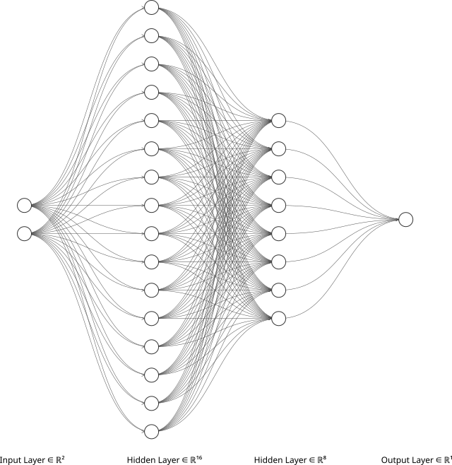
Visualization of the neural network we are making in this post. Image generated using this excellent tool.

Are there easier ways to learn a quadratic expression? Yes, but we’re building intuition for the immensely more complex neural networks that are used to model much more complex phenomena. The values for the sizes of the hidden layers are overkill, but still small enough to easily run, and having the number of neurons be a power of two is somewhat of a convention.

The learning rate is high compared to defaults for other state-of-the-art optimizers like Adam (which often uses a learning rate of 0.001), but it tends to work okay for simple problems.

During training, we perform 200 epochs. A single epoch is one pass through the entire training data set. I.e., if we have 300 data vectors, then, in one epoch, the model will see each of the vectors. After we perform backpropagation and update the parameters, we start the next epoch. We’ll take a look at the results in a bit, but by the time 200 epochs complete, we don’t really see improvement in prediction performance, so it makes sense to stop.

TorchLite Overview

TorchLite is primarily for understandability. It therefore doesn’t squeeze out performance, speed, or accuracy by adding tuning knobs that frameworks like PyTorch provide. That said, it does provide all the building blocks necessary to build a simple neural network.

• Tensors: data and gradients management. A tensor stores a data vector, the gradient for it (if any). It provides functions that let you perform math operations on the contained vector data, and is able to compute and store gradients as part of the backward pass.

• Layers and models: neural network base infrastructure. Building block classes include:

  • A Linear object is able to perform the linear transformations for all the neurons in a given layer (but not the nonlinear activation function),

  • Activation function classes like ReLU perform the nonlinear activation functions, and

  • A Sequential object is a container that can hold the pipeline showing the sequence that data will flow through. For instance, the network we are building in this post has this sequence: Linear (2 to 16 neurons) → ReLU → Linear (16 to 8 neurons) → ReLU → Linear (8 neurons to 1 neuron).

• Optimizers: code that defines how parameters in a neural network should be updated. The optimizer we’ve already looked at is stochastic gradient descent (SGD), where a w is updated with: w ← w - η × (∂L / ∂w), where η is the learning rate, and L is the loss computed when comparing the last prediction to the real outcome. There are other optimizers, too, such as Adam; we won’t get into the math here, however.

We won’t go into the code here, but you’re welcome to read it on GitHub.

Building and training the models

The PyTorch and TorchLite functions to make the models are fairly similar. This first code block is a small wrapper function that loads data, builds a model, and trains it. You can see the actual functions in main.py.

def train_network():
    # Load training data
    X_train, y_train = load_data('data/train.dat')

    # Create and train model
    model = MakeModel(input_size=2,
                      hidden_sizes=[16, 8],
                      output_size=1,
                      lr=0.01)
    model.train(X_train, y_train, n_epochs=200, log_interval=20)

    # Save training plot
    model.save_training_plot("outputs/torchlite_training.png")

    return model

Both frameworks build the same network. In TorchLite, Tensor, Linear, Sequential, and Adam are custom, minimal implementations; in PyTorch they come from the torch and torch.nn modules but behave the same way. See the TorchLite object in lite.py and the PyTorch object in full.py.

def __init__(self, input_size, hidden_sizes,
                   output_size, learning_rate):
        # Build the network
        layers = []
        prev_size = input_size
        for hidden_size in hidden_sizes:
            layers.append(Linear(prev_size, hidden_size))
            layers.append(ReLU())
            prev_size = hidden_size
        layers.append(Linear(prev_size, output_size))

        # Save network information for training and inference
        self.model = Sequential(*layers)
        self.optimizer = Adam(self.model.parameters(), lr=learning_rate)
        self.loss_fn = MSELoss()
        self.losses = []

Once we’ve defined the model, we run the training loop. Training consists of repeating three steps: forward pass to compute predictions and loss, backward pass to compute gradients, and an optimizer step to update parameters. We repeat this for the number of epochs we set (200 in our case).

def train(self, X_train, y_train, n_epochs):
    X = Tensor(X_train)
    y = Tensor(y_train)

    for epoch in range(n_epochs):
        # Forward
        pred = self.model(X)
        loss = self.loss_fn(pred, y)

        # Backward
        self.optimizer.zero_grad()
        loss.backward()
        self.optimizer.step()

        # Bookkeeping
        self.losses.append(loss.item())

At inference time, we just wrap the inputs in a tensor, pass them through the model, and read off the raw output values (i.e., predicted y values).

    def predict(self, X):
        X_tensor = Tensor(X)
        pred = self.model(X_tensor)
        return pred.data

Results

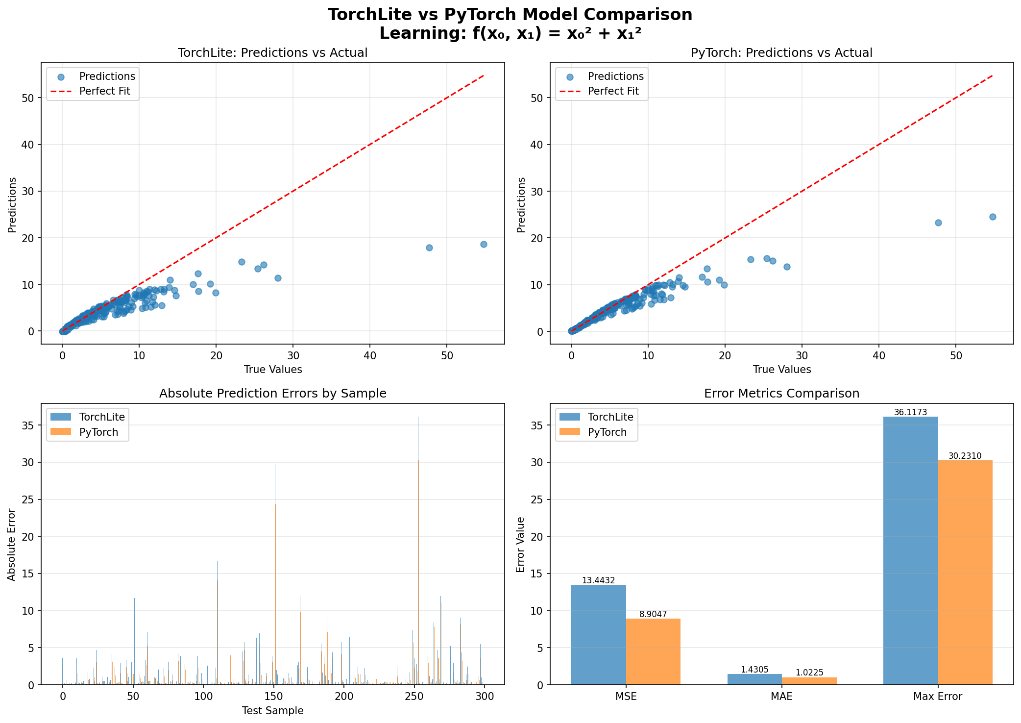
Both TorchLite and PyTorch learn the quadratic model decently well. PyTorch does a little bit better, but not that much better for this toy task. We can see the error for all the testing data (from test.dat).

Here, the top-left and top-right panels show the prediction accuracy of TorchLite and PyTorch, respectively, on all testing samples. The bottom-left panel shows the absolute error in prediction for both models (the interesting parts are the peaks, which are targets for improvement). The bottom-right shows the error each model achieved in aggregate. Performance is better when x₀ and x₁ are smaller, which we might be able to improve by increasing the amount of training data.

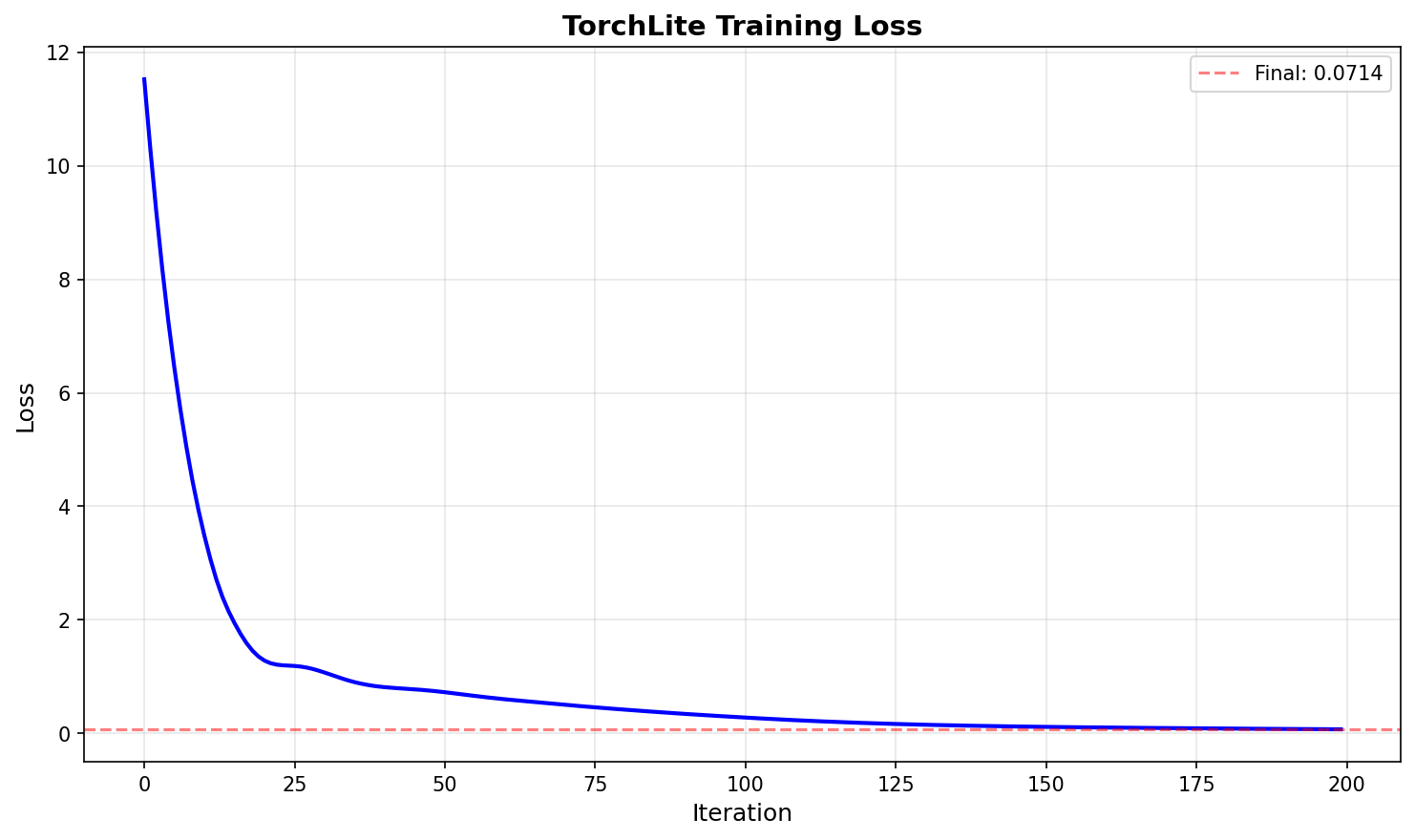
Now, let’s return to the earlier point about selecting the number of epochs. We used 200 epochs — was that enough? Below is the TorchLite training loss graph, where the x-axis shows epochs (also called iterations of the training loop). By the time we get to the 200^th epoch, we get little value by running another epoch. Even by the 150^th epoch, the diminishing returns likely mean it’s not worth the effort to run more epochs.

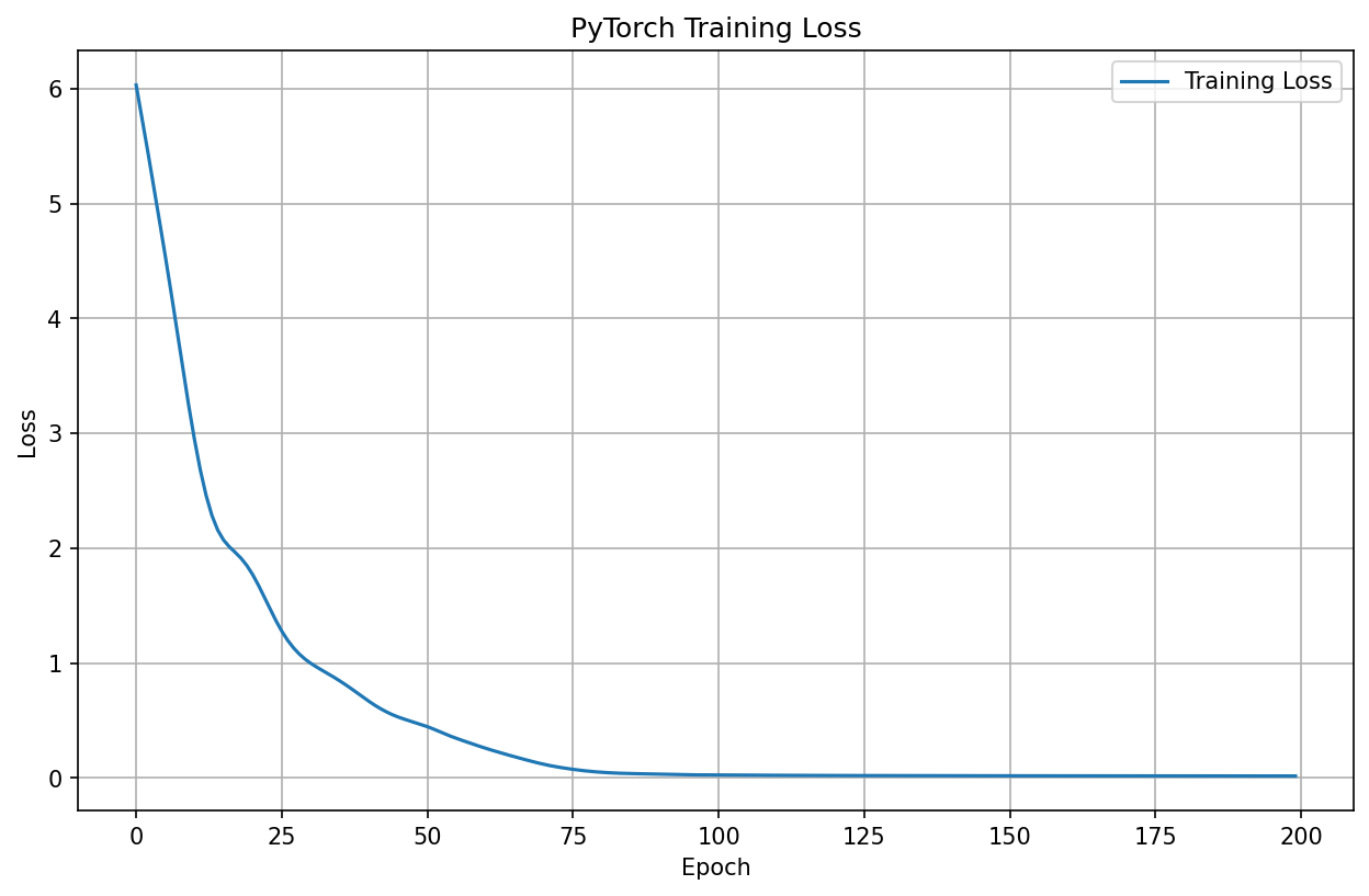
If we look at the PyTorch training loss in the below figure, it seems that it stops making improvements by the 100^th epoch, so we could likely have stopped training the model much sooner.

Recap

So both with TorchLite and with PyTorch, we’ve now built a simple neural network. TorchLite and PyTorch code looked surprisingly similar, but TorchLite’s simplicity lets us take a look at the infrastructure for a deep learning pipeline without all the optimization that PyTorch bakes in.

This is not the level of complexity needed for building a LLM, or even a small language model (SLM), but that was not our goal (yet). Hopefully, this post helps to map some of the theoretical concepts we’ve covered in the previous posts with a more grounded, hands-on toy project. Next, we’ll take a look at how to build something a bit more complex.

1. This is a bit different than the model that large language models (LLMs) use. LLMs have an output layer where you have a neuron per term in your vocabulary, and the value outputted from the neuron represents the probability the model assigns to that term being the next term that it should output, given the input. In this much simpler example, the neural network is directly predicting the value of y.