Ground-Up VLA: Optimizers and Learning Rate Scheduling

From GPU basics to robot foundation models

A few posts ago, we tried to build a model for the WikiText-2 dataset. Those models tended to have a high loss after training. To build more sophisticated models, in the previous post, we covered multi-head attention. Today, we’ll look into another concept that can help us build more sophisticated models: optimizers.

We’ve already introduced two optimizers in previous posts: stochastic gradient descent (SGD) and Adam. And we’ve covered the math of how SGD works. In reality, vanilla SGD is not the best choice for deep learning models, but it does provide a relatively simple starting point that builds intuition. Adam — and more recently AdamW — in combination with learning rate scheduling, is among the most common optimization strategies when building state-of-the-art deep learning pipelines.

What do optimizers do?

Let’s quickly review what role an optimizer plays in a deep learning pipeline. If we are given a batch of inputs in the matrix X, then we will perform a forward pass in the model that has a certain set of parameters (weights). Once the forward pass completes, we compute the loss to find how close the model got to correctly predicting the output associated with the input (e.g., predicting the next word of a sentence). Based on the loss, we want to update the parameters in the model.

Vanilla SGD computes the partial derivative of the loss with respect to an individual weight (but does this efficiently for all weights together via backpropagation), and subtracts the product of the learning rate and this partial derivative from the prior value of the weight. In more mathematical terms, w_new = w_old - α × (∂L / ∂w_old), where w_new is the new parameter value, w_old is the value of the parameter used in the last forward pass, α is the learning rate, and ∂L / ∂w_old is the gradient of the loss incurred with respect to the old parameter. More intuitively, the gradient tells us in which direction the weight should move if we wanted to increase the loss. Since we want to decrease loss, we move in the opposite direction.¹

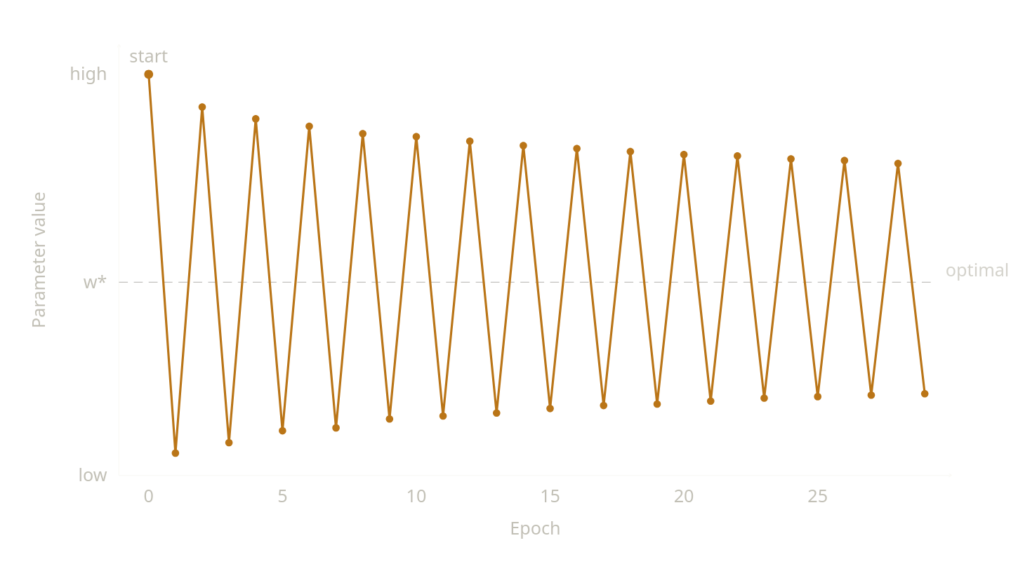
The problem with the basic parameter update rule that vanilla SGD uses is that it is very easy to end up with oscillation issues. You can end up in a weight thrashing scenario like below, where the parameter updates oscillate around the optimal weight value without ever actually settling on the optimal value.

SGD with Momentum

For those familiar with control theory basics, momentum introduces something like an integral term to the parameter update mechanism. Basically, we keep track of some history of where the gradient has been over some number of previous epochs. If we were to consider the loss landscape like a hilly terrain, and the gradient as an arrow that points us in a direction within this landscape, the momentum helps us nudge the parameter in directions that are more strictly in a downward direction than vanilla SGD, which might push the parameter in a mix of downward and sideways directions.

Parameter update rules based on momentum introduce a new term: velocity. Similar to how we track the parameter itself as w, we also track velocity v. The equations parallel what they do in vanilla SGD.

• v_new ← β·v_old + ∇L(w_old)

• w_new ← w_old - α·v_new

As before, α is the learning rate, but instead of directly updating the parameter with ∇L(θ), we update it using the velocity. The velocity, in turn, is what gets updated with the gradient. In effect, the velocity acts like an accumulator that will more strongly point in the direction that results in the best loss reduction as it accumulates more history of what gradients in prior epochs have looked like. The hyperparameter β, called the momentum coefficient, determines how influential the previous velocities are in determining the velocity for this epoch. In practice, β is typically set to 0.9, which has been empirically found to work well.

At first glance, it seems like we will continuously increase the velocity term, and it’ll grow larger and larger as the number of epochs increases. Let’s break down why that will not be the case so long as β < 1. The velocity term is a recursive equation. If we are currently on the k^th epoch, then the equation looks like the below.

• v_k ← β·v_k-1 + ∇L(w_k-1)

• v_k ← β·(β·v_k-2 + ∇L(w_k-2)) + ∇L(w_k-1)

• v_k ← β·(β·(β·v_k-3 + ∇L(w_k-3)) + ∇L(w_k-2)) + ∇L(w_k-1)

• v_k ← β^k·v₀ + Σ_i=0^k-1 ( βⁱ · ∇L(w_k-1-i) )

Since β < 1, each successive power of β shrinks, so older gradients contribute vanishingly little to the current velocity. The velocity remains bounded no matter how many epochs have passed. This is a geometric series with ratio β < 1, which converges to 1/(1−β), so if β=0.9, then with infinite epochs the multiplier term will be 10. This formally establishes that the velocity is bounded even over infinitely many epochs. It does seem a little odd, however, that the bounded multiplier effect we produce is up to 10x the gradient value. That is something that adaptive moment estimation addresses.

Adaptive Moment Estimation

SGD with momentum works remarkably well, especially for vision applications. Another common optimizer is called Adam, and more recently it has been supplanted by a variant called AdamW. At their cores, both of these optimizers combine momentum, which we just covered, with per-parameter-learning-rates. That is, instead of having a single value of α that we use for all parameters, we will track a separate α_w for each parameter w.

Mathematically, we need to restructure the parameter update to consist of three expressions, where there are two moment expressions—one for tracking gradient direction and another tracking gradient magnitude—that together are used to update the parameter. Let’s look at a simplified form of the math first, and then look at the full form.

• m_new ← β₁·m_old + (1 - β₁)·∇L(w_old)

• v_new ← β₂·v_old + (1-β₂)·(∇L(w_old))²

• w_new ← w_old - α·m_new / (sqrt(v_new + ε)).

The computation of wnew is actually slightly more complicated, as it is w_new ← w_old − α · m̂ / (sqrt(v̂ + ε)), but we’ll get to what the hat variants of m and v are after first walking through the simpler forms.

The first moment

The first expression looks a lot like how we described momentum in the previous section, with subtle differences. We have introduced a new multiplier (1 - β₁) to the term ∇L(w_old). As before, β₁ introduces exponential decay, so that the older gradients have progressively less influence on the moment m as the epoch number progresses. We now also have the multiplier term (1 - β₁) that applies directly to the gradient from this epoch. To see why, let’s revisit the geometric series we established at the end of the section on momentum.

We saw that, with momentum, if β=0.9, the accumulated gradient effect can reach up to 10× the magnitude of an individual gradient. This seems a little bit odd, since we have an effect that is quite a bit larger than the gradient’s magnitude. Let’s re-run the same recursive expansion with Adam to see what effect it has.

• m_k ← β₁·m_k-1 + (1-β₁)·∇L(w_k-1)

• m_k ← β₁·(β₁·m_k-2 + (1-β₁)·∇L(w_k-2)) + (1-β₁)·∇L(w_k-1)

• m_k ← β₁·(β₁·(β₁·m_k-3 + (1-β₁)·∇L(w_k-3)) + (1-β₁)·∇L(w_k-2)) + (1-β₁)·∇L(w_k-1)

• m_k ← β₁ᵏ·m₀ + (1-β₁)·Σᵢ₌₀^k-1 β₁ⁱ · ∇L(w_k-1-i)

The hyperparameter sums then turn into: (1-β₁) · Σᵢ₌₀^k-1 β₁ⁱ. As k → ∞, the bounded value of this geometric sum is 1. Now, in reality we do not have infinite epochs, so the sum after k epochs is 1 - β₁ᵏ. Therefore, Adam provides a bias correction factor by using the term m̂ = m / (1 − β₁ᵏ).

The second moment

The second expression we saw, v_new ← β₂·v_old + (1-β₂)·(∇L(w_old))², is how we track gradient magnitudes over time. That is, it doesn’t matter what the direction of the vector was, just what the magnitude of the gradient was. Parameters with large gradients get their learning rates downsized, while parameters with small gradients get their learning rates boosted. The math for the geometric sum of β₂ works the same as it does for β₁. And, like we computed m̂ = m / (1 − β₁ᵏ), we will also compute the bias-corrected v̂ ← v_new / (1 − β₂ᵏ).

When we compute w_new ← w_old − α · m̂ / (sqrt(v̂ + ε)), the effective learning rate becomes α / (sqrt(v̂ + ε)), which means that each parameter’s learning rate is adapted on the fly, but does not require us to store per-parameter learning rate hyperparameters.

Adam vs AdamW

What we’ve covered so far is Adam, but usually deep learning systems use AdamW now. The reason for the ‘W’ is decoupled weight decay. To understand what this does differently, we first need to take a look at how Adam computes loss.

Adam was developed when using L2 regularization was already standard practice, so practitioners continued to include the L2 penalty when computing loss: L_total = L + λ · ||w_old||² (see the post about regularization for more details). The downstream effect of this was that the regularization penalty became a part of the computed gradient ∇L(w_old), and the penalty correspondingly contributed to the computation of both the first and second moments of Adam. A parameter with large gradient history (large v) would get its weight decay dampened by the regularization partial derivative 2λw_old, and one with small gradient history gets its weight decay amplified. Adam is already doing manipulation of the weights, so you have something like a “too many cooks in the kitchen” effect, where the actions of L2 regularization are interfering with what Adam is supposed to be doing.

AdamW removes the application of L2 regularization from the loss computation, and instead applies the following at the time of parameter update: w_new ← w_old − α · m̂ / (sqrt(v̂ + ε)) − α·λ·w_old. This way, you get the weight decay effect without interfering in the moment computation.

Now, one question that arises is: isn’t there a decay effect already happening by application of the β₁ and β₂ hyperparameters in adaptive moment estimation? Not quite, because the Adam moment computations were decaying the influence of prior gradients, whereas the application of − α·λ·w_old decays the weight in this epoch. In other words, these are two different effects: one is a stateless decay applied directly to the weight, while the other is a stateful decay of gradient history within the moment estimates.

This decoupling of weight decay from adaptive moment estimation generally results in better generalization, so state-of-the-art systems tend to pick AdamW instead of Adam. For both optimizers, however, there is a related concept that is important in making them perform well: learning rate scheduling.

Learning Rate Scheduling

In addition to changing the optimizer, another way to deal with thrashing is to simply reduce the learning rate as a function of increasing epochs. To understand the intuition, consider how to play golf. You start very far from the hole, so you use swings with a lot of power to get the ball in the general vicinity of the hole. As you get closer to the hole, you reduce the power of the swings to achieve more precise control of the ball. Similarly, a larger learning rate is helpful in the early epochs of training, but as you get closer to the optimal weight, you want to achieve more granular control over how the parameters are getting updated.

Now, the analogy breaks down a little bit, because in golf you know where the hole is, but in deep learning you don’t know what the optimal weight is. In learning, we operate on the assumption that after some fixed number of epochs, we will be in the right vicinity of the optimal weights (otherwise we have a model that generalizes poorly). If we were to modify the golf analogy, it would look like the following scenario:

• I don’t know where the hole is, but I know that I can get distance-to-hole estimates after each swing.

• I’ll preplan my swings so that high-power swings are near the beginning, and low-power swings are at the end, on the assumption that I will have used the early swings to get much closer to the hole.

There are many ways that these learning rate schedules are generated. The below graph shows some of the common approaches, with the baseline being a fixed learning rate over the course of the entire training sequence.

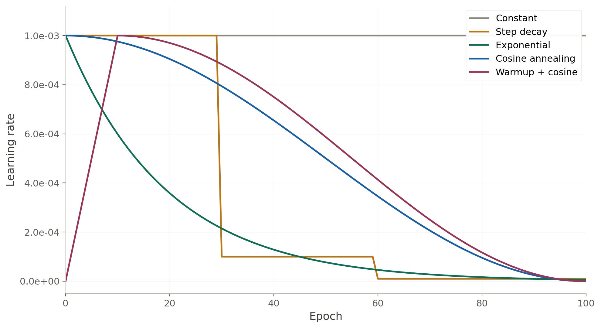
In practice, cosine annealing and warmup + cosine are the most often used for transformer-based deep learning. The reason for a warmup phase that ramps up the learning rate is that since we have no idea where optimal weights will lie or even in what direction parameters should move, the gradients can swing wildly. If we give the beginning of training to this warmup period, that lets the training naturally find, very broadly, what directions parameters should be moving in. After the warmup, we can be a little more confident that the steps we take to update parameters will be in the right direction.

Recap

Today, we’ve covered some of the last important conceptual pieces needed to build a sophisticated LLM. We reviewed vanilla SGD and what its weaknesses are, introduced momentum, covered both Adam and AdamW, and covered the intuition of learning rate scheduling.

This brings us to a point where we can start looking beyond text to vision; rather, how vision and text are used together in models capable of reasoning about images. As a precursor step, we’ll take a look at how vision and text are combined by the application of a new type of attention: cross-attention.

1. This is remarkably similar to proportional control in control theory.