Ground-Up VLA: Model Depth and Width

From GPU basics to robot foundation models

Last time, we built a small neural network that learned to approximate a quadratic function, predicting a numeric output from a numeric input. This is a classic regression setup, because the model outputs a continuous value.

This time, we’ll switch to predicting tokens instead of numbers: given some text, we’ll predict the next token in a sequence. That moves us into the language modeling world, where the task is framed as a sequence of classification problems over a vocabulary.

To do this, we’ll build a tiny language model and wrap it in a simple training and inference pipeline that includes a transformer layer. We’ll look at two hyperparameters —model depth (number of transformer blocks) and model width (d_model) — and see how far they get us in producing a model that reasons about text.

Intuitively, model width increases provide the model with more dimensions to represent individual tokens at each layer of the model. E.g., at a particular layer, a model might be thinking about the type of concept the word ‘bank’ is representing: it could be either a financial institution or a riverbank, and future layers will rely on the nuance that this layer of the pipeline establishes.

In contrast, depth gives the model more sequential steps of reasoning. A deeper pipeline might have later layers that build on the understanding that 'bank' represents a financial institution. But that reasoning is only possible because an earlier layer established the distinction — if the pipeline ended there, the model couldn't take the next inferential step.

Problem Overview

We’re going to train a tiny transformer language model on the WikiText-2 dataset. The task is next-token prediction: given a sequence of tokens x_<t​, predict the token x_t that comes next.

For example, if the text contains:

“The quick brown fox”

then we train the model to answer questions like:

• context: “The” → predict: “quick”

• context: “The quick” → predict: “brown”

• context: “The quick brown” → predict: “fox”

At every position (time step) t, the model outputs a vector of logits over the vocabulary; after softmax, this becomes a probability distribution p(x_t∣x_<t). We train by minimizing the loss over all tokens in the training set. We evaluate on a held-out validation set and final test set. The evaluation can be done by looking at the loss or the perplexity (a metric that is directly derived from loss, and one which we won’t examine in detail here).

Even with a small model, we can observe how architectural and training hyperparameters—such as model width (d_model) and model depth (number of transformer blocks)—affect training dynamics, overfitting, and validation perplexity.

To solve this, we will build four components:

1. Vocabulary builder: create integer IDs for all the different elements in the WikiText-2 dataset. I.e., generates a static map of natural language elements (like ‘habanero’) and integer IDs (like ‘3’).

2. Tokenizer: Converts text to IDs and IDs to text. This is different than a vocabulary builder because it does this conversion for a particular input sequence; given a sequence like ‘habaneros are not spicy enough’, the tokenizer will refer to the vocabulary produced by the vocabulary builder and output an integer sequence like [3, 1, 5, 3, 4].

3. Dataset loader: Loads the data files, splits into training, testing, and validation sets.

4. Transformer model: The actual deep learning pipeline that will interpret our natural language and, given a text sequence, try to predict what the next part of the sequence should be.

Data Setup

The dataset for the Wikitext2 dataset is available via a Python library from HuggingFace. The first thing we will do is build a vocabulary. Each vocabulary provides a bidirectional map between a token (like “find”) and an ID (like “1”).

A tokenizer is used before and after data passes through the deep learning pipeline. When used prior to the pipeline, the tokenizer is used to encode natural language to IDs using the vocabulary we’ve made, which the model will then convert to embeddings. When used after the pipeline, the tokenizer will decode the selected “most likely next token” from a token ID¹ to an element of the natural language vocabulary we have available.

The dataset loader handles splitting the data into parts so that we have different training, testing, and validation sets of data. The training set is used during the training loop, where parameters can be updated. The testing set is used to determine how the model behaves on data it was not trained on. The validation set, also called the dev set, can be treated like a tuning set: we use it to choose or adjust configuration parameters of the model (hyperparameters), such as learning rate or model size, while developing the model.

Modeling

Next, let’s build the model. At this point, unlike with the previous post, we will move to fully using PyTorch — the complexity of the models becomes too large for our easier-to-understand TorchLite framework. Since we are now building a language model, we’ll make a few adjustments compared to the regression task we performed in the previous post.

1. We have already discussed how the output layer now consists of one neuron per element in the vocabulary. (The model produces logits over the vocabulary; after applying softmax, these become probabilities.) The deep learning pipeline will produce a probability distribution as its output. Each probability corresponds to the model’s answer to the question “How likely is it that this element of the vocabulary is the next token in the output sequence?” One simple way to interpret this information is to take the element with the highest probability and output that as the next output token.

2. To perform the probability-based selection well, models typically do not use a loss based on Euclidean distance, which is what we used in the previous post. They instead use cross-entropy loss. We’ll take a look at what this means before diving into the model.

3. There are a few other concepts that start playing a role now: batch size, regularization, and multi-head attention. We won’t tackle these concepts here, and instead leave them to a future post. Just note that we will use a fixed batch size, thereby allowing a model to look at multiple sets of (input, output) pairs in parallel.

Cross-Entropy Loss

Recall that the loss represents how surprised the model is by the correct answer. The first type of loss function we looked at was mean-squared error: we computed the squared Euclidean distance between the predicted and the true vectors. For instance, if we are given y_true and y_pred, then L = || y_true - y_pred ||₂².² In classification tasks, which is what this post’s language model performs, we typically use cross-entropy loss.

Assuming that there is only one “correct answer” for what element from the vocabulary should appear at position t of a sequence, the cross-entropy loss looks like the following: L_cross= − log p( y_t∣x_<t ). Let’s break this down.

Suppose we have a text sequence S = [s₁, s₂, …, s_T]. Each element of S represents a specific token ID and is in the vocabulary space V. E.g., s₁ might have value 3 and map to the word “hello”. s_t is the ground-truth token ID at position t; y_t is just s_t, but we use a different symbol to emphasize that it’s the label at time step t. The probability of the model selecting the correct value y_t is based on all the tokens of S that preceded it; in other words, x_<t = [s₁, s₂, …, s_t-1].

Let’s ground this abstract math with a concrete example. Suppose the sentence was “habaneros are not spicy enough.” Then, at time step t = 4, these are the assigned values:

• Vocabulary: [ are=1, habaneros=2, spicy=3, enough=4, not=5 ]

• S = [ s₁ = 2, s₂ = 1, s₃ = 5, s₄ = 3, s₅ = 4 ]

• For t = 4

  • y₄ = s₄ = 3.

  • x_<t = [ s₁ = 2, s₂ = 1, s₃ = 5 ]

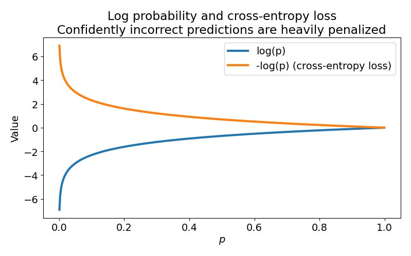
The value p( y_t∣x_<t ) = p( ‘spicy’ | ‘habaneros are not’ ) would then represent the likelihood that, at time step t = 4, the model predicts the output to be “spicy”, given that the previous components of the input sequence formed “habaneros are not”. If the model predicted high probability for y_t being the next token in the sequence, then the loss must be low. The log of an input in the range (0, 1] is nonpositive, hence why we compute -log. This is illustrated in the below figure. As p(y_t∣x_<t) approaches 1, the loss −log⁡ p(y_t∣x_<t) approaches 0; as it approaches 0, the loss grows without bound.

Model Architecture

Now that we’ve established the loss function, let’s figure out how to build the deep learning pipeline. As with state-of-the-art models, we’re going to use stacked transformers.

The input is going to be a text sequence, and the output will be the next token that should be present in that sequence.

• Input: Text sequence

• N Transformer Blocks, where N is in the set { 1, 2, 4, 8 }

• Output: The next element of the text sequence

I initially tried to keep this on my laptop, but partway through an attempted training, the thermal protection kicked in and the laptop shut off, so I switched to Colab. This architecture in and of itself should hopefully make sense given the previous posts in this series, but there are many ways to tune its performance and behavior. In the next section, we’ll start exploring how different hyperparameters affect the loss.

Experiments

In this section, we’ll run two types of experiments and see what effect they have on the model loss. The first will be varying the model depth (number of transformer blocks). The second will be to fix the depth and vary the model width (d_model). The main goal of this exercise was to see how these two hyperparameters affect how close the model gets to producing good output text sequences. The closer a model gets to producing a sentence we could conceive of appearing in a wiki article, the lower the loss should be.

Model Depth

The general idea I’ve heard is that modern LLMs are all about very deep pipelines. So, naturally, my first inclination was to look at how model depth affected loss. I picked the following model hyperparameters:

• d_model = 256

• d_ff = 4 d_model

• Batch size: 32

• Learning rate: 0.01

• Number of epochs: 20

• Number of transformer blocks (independent variable): [1, 2, 4, 8]

Let’s approach this in pieces.

Number of Parameters

When we train the different-depth models, we expect the number of parameters to increase with depth. This should be a linear relationship, since each transformer block adds a fixed number of additional parameters. And this is what we observe.

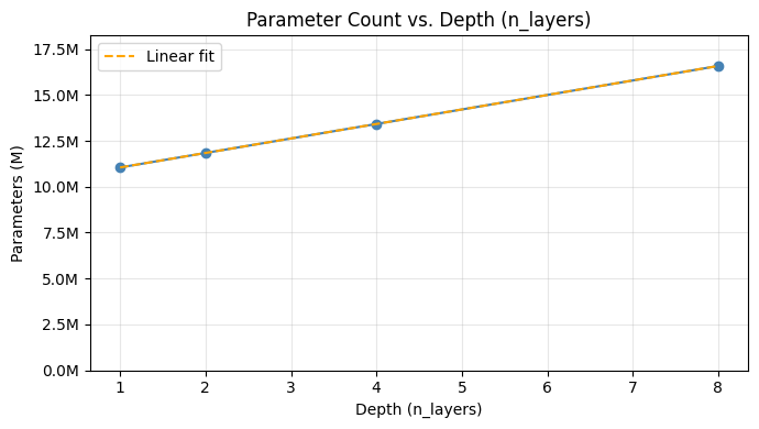
The number of parameters in the model has three components to it.

1. The embeddings, which are a function of the vocabulary size and model size: |V| * d_model.

2. The outputs, which are also a function of the vocabulary size and model size: |V| * d_model.

3. The number of transformer blocks: N x P_block, where P_block is the number of parameters per transformer block.

Loss vs. Number of Transformer Blocks

Next, let’s take a look at how the loss changes as a function of the number of transformer blocks. Recall that our simple hypothesis was that the loss should decrease as a function of model depth.

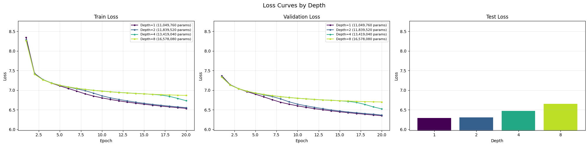
We observed that training loss and validation loss both tended to go down, but the test loss went up. The rising test loss alongside falling training loss suggests the deeper models are beginning to overfit, where a model starts to adapt to the specific dataset that was provided as training input and is unable to generalize to examples it does not see in training. At a model depth of 8 transformer blocks, we also start seeing the validation loss remain higher by epoch 20 than the shallower models, which seems to support the overfitting claim.

It’s still possible that we’re not overfitting, but rather underfitting, and we just need to use more epochs or deeper models before we start to see the benefits of more complexity. We’ll revisit this possibility after we look at our next set of experiments.

Next, let’s examine a different independent variable to see if it helps: model width.

Model Width

Let’s fix the model depth at four transformer blocks. And, as per general recommendations, we’ll also fix d_ff = 4d_model. That means our independent variable is now d_model.

• Model width: d_model = [64, 128, 256, 512]

• d_ff = 4 d_model

• Batch size: 32

• Learning rate: 0.01

• Number of epochs: 20

• Number of transformer blocks: 4

Number of Parameters

As we did for model depth, let’s take a look at how the number of parameters grows as a function of the model width. A regression analysis shows us that the parameter increases quadratically rather than linearly, in contrast to what it was for model depth. Where is the nonlinearity coming from?

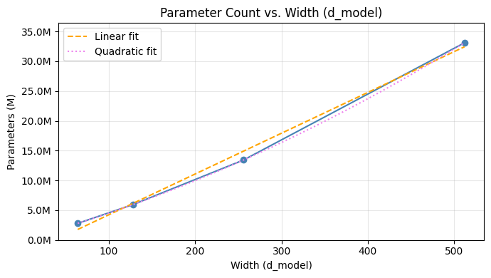
Previously, we considered three factors affecting total number of parameters: the embeddings (|V| * d_model), the outputs (|V| * d_model), and the number of transformer blocks (N x P_block). Clearly, changing d_model will affect the embeddings and outputs, but that is not a nonlinear relationship. For that, we have to look into P_block.

Each transformer block consists of a self-attention sublayer and a feed-forward sublayer. Both types of sublayers have weight matrices that represent trainable parameters.

• Self-attention sublayer: We compute Q = XW_Q, K = XW_K, V = XW_V, and then apply an output projection W_O.³ Each projection matrix W_Q, W_K, W_V, and W_O is typically of size d_model x d_model. Therefore, the number of parameters in this layer grows at the rate O(d_model²). See the self-attention post for more details.

• Feed-forward sublayer: The feed-forward network within this sublayer consists of two linear layers that move embeddings from dimensionality d_model → d_ff → d_model. This requires matrices of size d_model x d_ff and d_ff x d_model. Since a common value of d_ff = 4 d_model, the number of parameters in this layer also grows at the rate O(d_model²).

Loss vs. Model Width

Next, let’s observe how the loss changes when, instead of varying the model depth, we vary the model width.

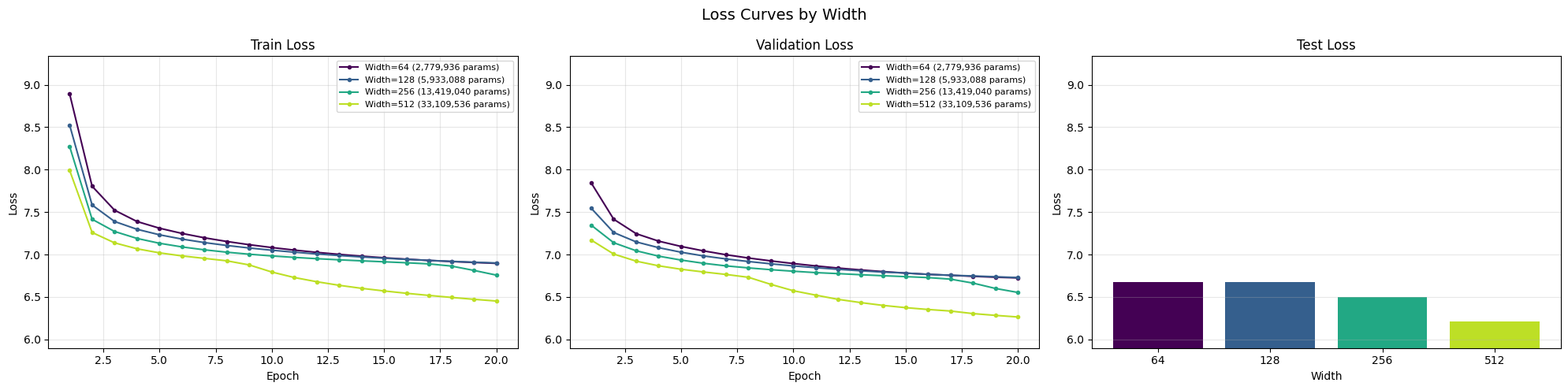
We see an interesting trend that is somewhat opposite of what we observed for depth: increasing model complexity is consistently driving down training, validation, and test loss. Since we have way more parameters in the model width experiments than in the model depth experiments, this might indicate that our model depth experiments were not overfitting the data, and we might want to, e.g., consider training the deeper models for more epochs.

However, this is still not an airtight argument. As we mentioned at the start of this post, model width and depth affect a model’s ability to reason about any given topic in different ways. This also confirms a result that others have also observed: for small pipelines, increasing model width has outsized impact on lowering loss as compared to model depth.

Recap

This was a somewhat long post, but we covered important ground. We introduced our first real transformer model, and examined the effects of two hyperparameters on the loss incurred by this model on the WikiText-2 dataset. We explored why model depth has a linear relationship—and why model width has a quadratic relationship—with the number of parameters.

We observed that model depth is not the end-all-be-all in determining how well a model performs, since our wider models could better drive down loss than our deeper models. Similarly, there are many hyperparameters that can be tuned to improve a model’s ability to generalize. Next time, we’ll start exploring a few more such methods: batch size and regularization.

1. A single neuron corresponds to a single item in the vocabulary. So, if we have a 512-word vocabulary, then the output layer will have 512 neurons, each directly mapping to a particular token ID, and therefore a particular element of the vocabulary.

2. The previous post’s notation avoided squaring the Euclidean distance, which is atypical when this type of loss is used.

3. We called W_O the matrix A in the self-attention post, but W_O is a bit more descriptive.