Ground-Up VLA: Batch Size and Regularization
From GPU basics to robot foundation models

Last time, we started investigating our first real transformer model based on the WikiText-2 dataset. We examined two hyperparameters: model depth and model width. Both these hyperparameters tend to increase model complexity as they increase in value. Today, we’ll look at techniques that reduce model complexity, which can result in models that generalize better.
Specifically, we’ll be looking at the effects of batch size and regularization, where regularization will be broken down into a few types of hyperparameters: L1 regularization, L2 regularization, and dropout rate.
We’ve already introduced batch size as a means by which to let a model examine multiple input sequences in parallel, but it has knock-on effects on model complexity due to how it affects loss computation.
Note: I kept running out of compute resources in Colab as I tried different variants of the setup to see the effects of regularization, so I made a VM in Thunder Compute and ran there ($0.27 / hr). I’ve added a setup script to the repository that you can use for your own setup.
Batch Size
Batch size answers the question:
How many training examples do I look at prior to updating parameters once?
In the simple y = f(x) view, we often think of updating the model using a single input–output pair at a time. Batching extends this idea to many examples at once. We define a batch X = [x1, x2, x3] and corresponding targets Y = [y1, y2, y3], and pass all of X through the model in parallel to predict all elements of Y.
A bit more concretely, let’s consider a dataset consisting of two examples:
“list mango varieties” → “Alphonso, Badami”1
“show me vacation ideas” → “Tokyo, Mumbai, Paris, New York City”
When batch size is one, we will pass the example of “list mango varieties” through the pipeline, compute the loss on how close the model got to predicting “Alphonso”, a comma, and “Badami”.
When batch size is two, we pass both “list mango varieties” and “show me vacation ideas” to the pipeline at once, and loss is computed. This will mean we have two losses, one for the “list mango varieties” example and another for “show me vacation ideas”. We compute the batch loss (Lbatch) as the average of the loss for all examples in the batch. Backpropagation will then try to find ∂Lbatch / ∂w rather than the example-specific partial derivative ∂L / ∂w.
The normal cross-entropy loss for a non-batched input sequence would look like the following:
For an input sequence of size T, we ask how well the model predicted each token in the sequence. When we have a batch consisting of B input sequences, the loss changes to a sum over the losses of each input sequence in the batch.
A larger batch means we can perform more parallel computation (because all examples are processed simultaneously by the GPU), and we tend to perform parameter updates that reduce the average loss rather than the loss of any individual example. And, the larger the batch is, the fewer times we perform weight updates, since we do a full forward pass on the entire batch before doing a round of weight updates.
Let’s see what this looks like in practice. Using the same WikiText-2 dataset from the last post, the below graph shows a parameter sweep across the batch sizes of 8, 16, 32, 64, and 128. As the batch size increases, the test loss is continuously increasing, although the training loss is continuously decreasing and validation loss is also usually trending lower. Why is batch size 8 so much better than batch size 128? Well, if we had a total of 256 input sequences to train on, then a batch size of 128 means we update the weights 2 times (two forward passes per epoch), whereas a batch size of 8 means we get to update the weights 32 times per epoch. This means that the model is able to tune its weights more with a smaller batch size.
All the models can be counted as ‘converging’ because the training and validation losses are still decreasing. However, we are starting to see diminishing returns per epoch by the 20th epoch, and the larger batch sizes are consistently performing worse.
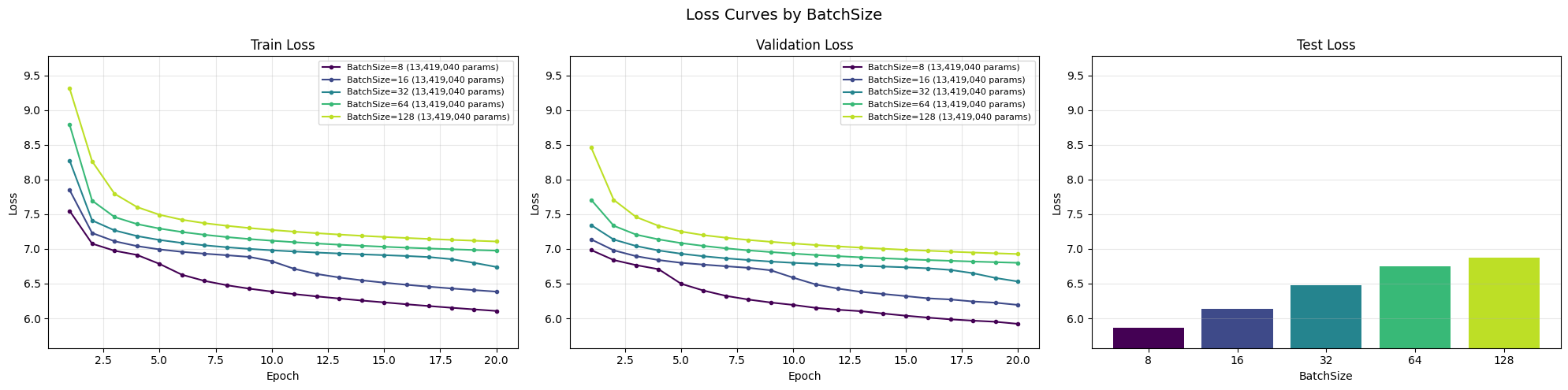
More broadly, a small batch size means each weight update is based on very few examples, making the gradient estimate noisy. This noise acts as implicit regularization — it prevents the optimizer (in our case, stochastic gradient descent) from confidently committing to sharp, narrow minima and instead tends to find flatter regions of the loss landscape that generalize better.
This might lead us to the deduction that we’d ideally have batch size 1, since this will maximize the model’s exposure to noise in the gradients that are computed. However, there is a risk: at some point, the exposure to additional noise makes it difficult for a model to find any optimized set of weights to converge to, and results in weight thrashing, where a model switches back and forth between various minima it finds, which will then generalize poorly. Additionally, a batch size of one is not computationally practical, since every input sequence will perform a full set of parameter updates before the next input sequence can be examined, thereby negating much of the parallelism advantage that a GPU provides.
Regularization
Regularization refers to a set of techniques that are used to reduce model complexity. The concept is extremely useful to prevent overfitting of models. In other words, models get quite good at adapting weights to the specific examples you give them for training, and this can result in poor test-time performance when the input does not match what was seen at training time. That said, as we’ll see in today’s experiments, regularization on its own is sometimes not what unlocks amazing generalization, and instead needs to be paired with some other complementary concepts (e.g., learning rate scheduling).
Today, we’ll look at L1 regularization, L2 regularization, and dropout rate. Examples of other techniques include elastic nets, label smoothing, early stopping, and data augmentation2. We’ll briefly touch on early stopping because it will naturally show up in the graphs we look at.
L1 Regularization
With L1 regularization, we modify what loss value is used for backpropagation. We apply a penalty that is added to the simple cross-entropy loss. This involves introducing a new hyperparameter λ, which controls the strength of the L1 regularization penalty.
Recall that in backpropagation, we compute the derivative of the loss with respect to a given weight wj.
For a given weight wj, the update step involves subtracting the gradient for that weight from the prior value of the weight.
So if wj > 0, then sign(wj) = 1 and you will be subtracting a positive value from a positive value, which will push the new wj closer to zero. If wj < 0, then sign(wj) = -1 and you will be subtracting a negative value from a negative value, which will again push the new wj closer to zero.
More intuitively, L1 regularization will push weights that are very small to eventually acquire a value of 0, while large weights will not reach 0. This has the effect of selecting for those features that are most important. To take a more practical example, if the model is building an understanding of carpets, then there might be two factors to consider: thread type and ambient temperature. Ambient temperature might play some role in determining how comfortable you feel on the carpet, but is not nearly as important to understanding carpets as thread type. L1 regularization, ideally, would make the model not need to think about the ambient temperature when thinking about carpets.
In practice, pure L1 regularization is generally not used in very deep pipelines, where small weights still play some role in helping the model understand subtle nuances of topics. But it can be useful in combination with other techniques and for certain specialized model types. For the sake of simplicity, we won’t get into combination regularization techniques today, but if you want to read more, you can look up elastic nets.
Now, let’s take a look at a practical example. Continuing with our WikiText-2 dataset, let’s perform a hyperparameter sweep experiment where we vary the value of the L1 strength λ across the set [0.0, 1e-8, 3e-8, 1e-7, 3e-7, 1e-6]. We can see how the hyperparameter impacts the loss as below:
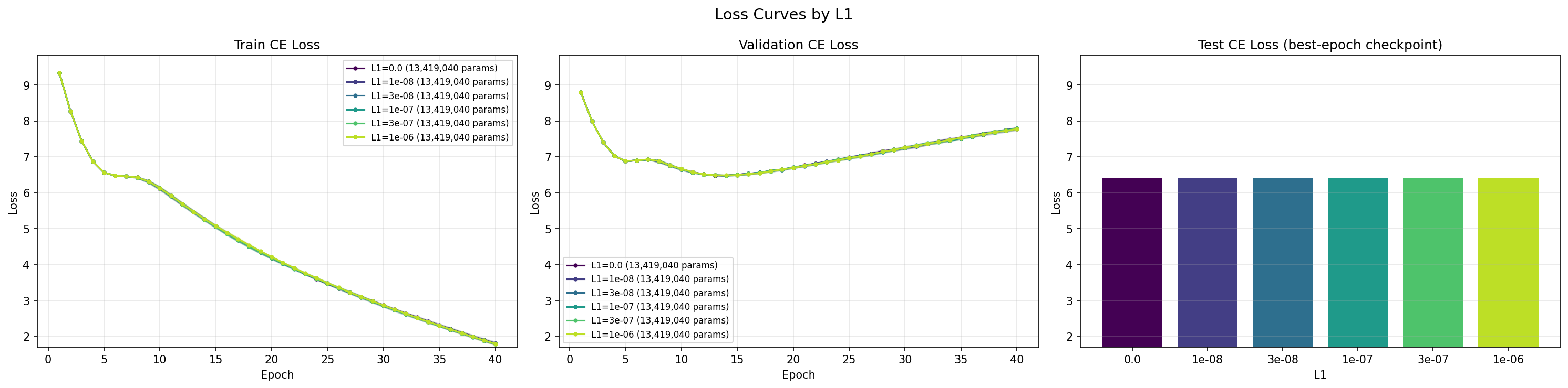
We see that training loss pretty uniformly goes down as we train for more epochs, regardless of the value we set for λ. That is not the trend we see in validation loss. Around Epoch 5 validation loss hits a minimum, after which it starts to tick up before decreasing again around Epoch 8, and finally switching to steadily increasing values after around Epoch 14. This demonstrates how finding an optimal set of weights is not a linear process, and sometimes you do need to simply persist to make your way out of a local minimum. At the same time, the more you train, the more likely it is that your model becomes overfitted to your training data and does not generalize well to data it has not yet seen.
If you train for enough epochs, however, you should be able to see where your model generalized the best, and simply take the weights from that epoch and claim that as the trained model. This is exactly what early stopping means.
Of course, even with early stopping, we don’t really see any change in the test loss. We might as well have not done the regularization and saved ourselves some computation. This broadly tracks with what people do in practice: state-of-the-art deep learning architectures usually don’t use L1 regularization because L2 regularization has been found to work much better. (Spoiler: L2 is also not that helpful for what we build in this post, but we’ll introduce the concept because we need it to build on for when we get to more complex models where it is helpful.)
L2 Regularization
L2 regularization is quite similar, conceptually, to L1 regularization. It relies on applying a penalty to the cross-entropy loss. Instead of the penalty being proportional to the absolute value of weights, however, the penalty is proportional to the square value of weights.
This has the downstream effect of changing what the gradients look like.
And this, in turn, affects how individual weights are updated.
Due to each weight update now including the term wj(1 - 2λη), this is also known as weight decay. Large weights get penalized more heavily than small ones, and weights are not pushed directly to 0 values, but are “nudged” in that direction, since the weight update delta gets weaker the closer the weight gets to 0. More intuitively, a model should spread the responsibility of understanding throughout all the neurons it has available, rather than allowing individual neurons to take decisions on the meaning (i.e., have 5 neurons together determine whether we are talking about ‘bank’ as a financial institution or a riverbank). This is supposed to improve how robust a model is to small changes in input (e.g., when a person says they do their banking down the street, the model understands the person uses a bank at the end of the street rather than does something on a riverbank).
L2 regularization is quite common in deep learning pipelines because it is simple, stable, and effective across a wide swath of architectures.
So, what does it look like in our pipeline? Let’s see below.
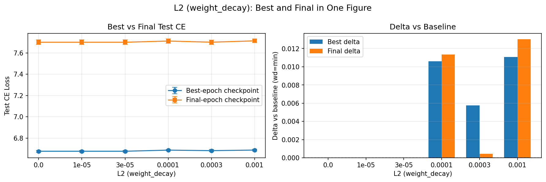
Well, that’s odd. It looks pretty similar to the results for L1 regularization, in that it’s not very impactful. Even if we use early stopping, there’s barely any impact on test loss when compared with the no-regularization scenario.
In practice, the effectiveness of L1 and L2 regularization depends on several other factors. E.g., the dataset you use, co-tuning the hyperparameters with other hyperparameters like learning rate, and model complexity all affect how useful L1/L2 regularization will be. See the Stanford CS231n notes on regularization, this Geeks for Geeks article, or this MachineCurve article for more. We’ll also return to this in a future post.
Dropout Rate
Dropout rates are a very different type of regularization than L1 and L2 regularization. If you’re interested in details, check out the original paper, but we’ll briefly cover the math here. Instead of modifying the loss function, dropout is used during the forward pass of a model undergoing training. While the model is undergoing training, every neuron has some chance of producing a 0-value output with a certain probability for a given forward pass of data flowing through the network.
A bit more explicitly, we can say the following.
The effect is that the model avoids single points of failure by distributing responsibility for reasoning across many neurons.
There is one aspect of this equation that warrants a little bit of investigation: Why do we have hi / (1 - p) rather than just hi? This has to do with how dropout affects future computation. At test time, since there is no dropout, every neuron can contribute its understanding of an input token to neurons of the next layer.
If we train the system under the conditions that 10% of inputs are zero, then this will affect how a future neuron reasons about the inputs it receives; i.e., at test time the linear combination of the outputs from the previous layer might be 1.2, but when doing training with dropout they might be 0.9 (for the same input sequence). By scaling hi by the factor 1 / (1 - p), we ensure that future neurons continue to base their reasoning on inputs that are in the same range as it would actually receive at test time.
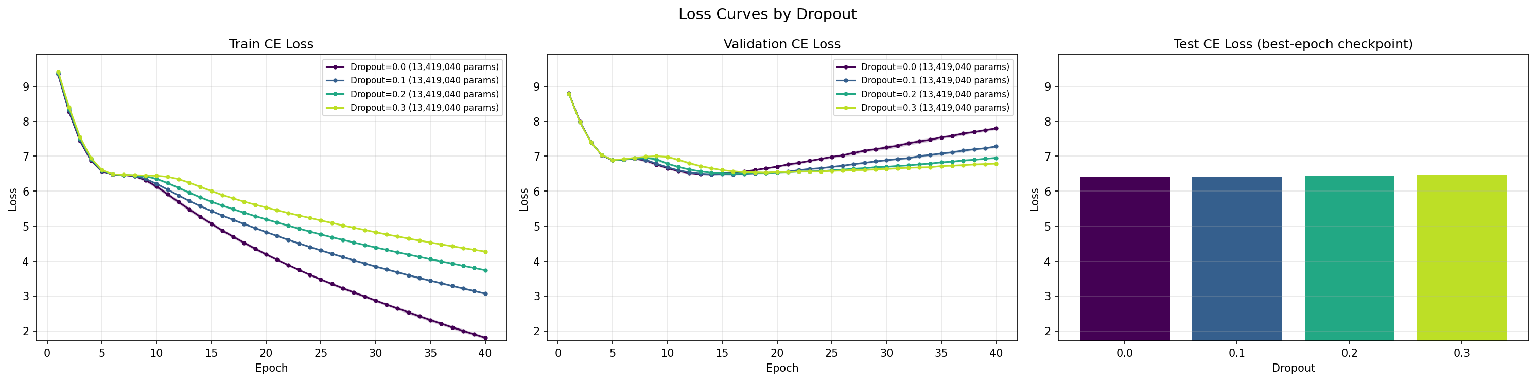
Let’s take a look at how dropout affects loss in the WikiText-2 dataset. Here, the effect of dropout is somewhat more clear when comparing training and validation loss. The case with no dropout adapts to the training set much more rapidly than setups with dropout, as we see that 0-dropout loss getting to a much lower value by the end of the 40 epochs than any other loss, which all contain dropout. Additionally, the validation loss curve rises more rapidly for the 0-dropout case than any others.
However, as before, we don’t really see an effect on the test loss. The graphed test loss is for the “best epoch”, which is the epoch of training that produced the best generalization. This is pretty early on, around Epoch 7, and the training/validation loss lines have not started to diverge at this point, so it makes sense that test losses are roughly comparable in value. After Epoch 7, however, we see that regularization does prevent the models from overfitting as aggressively to the training data.
Recap
Today, we covered batch size and three types of regularization: L1, L2, and dropout. We took a look at the math behind the techniques and a brief glance at the impact each of them produces on the WikiText-2 dataset that we started using as an example in the previous post.
We took a look at how smaller batches tend to be better for generalization, since they introduce more noise into the training, but we generally do not want to go to batch sizes of 1 due to both weight thrashing concerns and the loss of parallelization that comes with such small batch sizes.
We saw how L1 regularization works, and why it tends to push many weights to 0 values. L2 regularization, in contrast, tries to distribute responsibility of interpretation amongst many neurons by never pushing weights to be exactly 0. In the experiments we ran, today, however, neither approach seemed to provide immense benefits. We’ll investigate this further when we look into complementary techniques like learning rate scheduling.
Dropout, in contrast, was able to show us the benefits of regularization. Without dropout, the validation loss grew much more rapidly, and the training loss decreased more rapidly, than the counterpart models that did use dropout values greater than zero.
Now, we will want to further investigate how L1 or L2 regularization can help, for which we will need to investigate more complex models on, perhaps, more complex datasets. To do this, we will first need to go over a concept we mentioned but didn’t explain in a prior post: multi-head attention. So, we’ll cover that in the next post, followed by some more information on the other ‘parts’ we need to understand to build more complex models, before actually building the complex models and revisiting regularization.
There are many more types, but we’ll keep the example small.
Arguably, data augmentation is not a type of regularization. This involves inflating your training data by performing transformations on an input. For instance, given a cat picture you zoom in, zoom out, rotate 30 degrees, rotate 60 degrees, etc., and use each of these as a new input that the model should learn to classify as ‘cat’. However, sometimes this is counted as regularization because it reduces overfitting error.